It is the process of grouping documents such that documents in a cluster are similar and documents in different cluster are dissimilar. Vector space model is used.
Algorithm
- Choose the value of k
- K objects are randomly chosen to form centroid of k clusters
- Repeat until no change in location of centroid or no change in objects assigned to cluster
Find distance of each object to cluster center and assign it to one with minimum
Calculate mean of each cluster group to compute new cluster centers
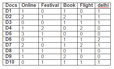
Let k=3 an initial cluster seeds be d2, d5 and d7.
calculating Euclidean distance between d1 and d2 :
The clusters are:
d2, d1, d6, d9, d10
d5, d8
d7, d3, d4
If you want something and you get something else, never be afraid. One day things will surely work your way!!
Google AIY Vision Kit
Google has introduced the AIY Voice Kit back in May, and now the company has launched the AIY Vision Kit that has on-device neural network acceleration for Raspberry Pi. Unlike the Voice Kit, the Vision Kit is designed to run the all the machine learning locally on the device rather than talk to the cloud. While it was possible to run TensorFlow locally on the Raspberry Pi with the Voice Kit, the previous kit was far more suited to using Google’s Assistant API or their Cloud Speech API to do voice recognition. However the Vision Kit is designed from the ground up to run do all its image processing locally. The Vision kit includes a new circuit board, and computer vision software can be paired with Raspberry Pi computer and camera.
In addition to the Vision, users will need a Raspberry Pi Zero W, a Raspberry Pi Camera, an SD card and a power supply, that must be purchased separately. The Kit includes cardboard outer shell, the VisionBonnet circuit board, an RGB arcade-style button, a piezo speaker, a macro/wide lens kit, a tripod mounting nut and other connecting components.
The main component of the Vision Kit is the VisionBonnet that features the Intel Movidius MA2450 which is a low-power vision processing unit capable of running neural network models on-device. The software includes three models:
- Model to recognize common objects
- Model to recognize faces and their expressions
- Person, cat and dog detector
Google has also included a tool to compile models for Vision Kit, and users can train their own models with Google’s TensorFlow machine learning software. The AIY Vision kit costs $44.99 and will ship from December 31st through Micro Center. This first batch is a limited run of just 2,000 units and is available in the US only.
AWS Deeplens
Amazon’s Deeplens device introduced at Amazon ReInvent is aimed, at software developers and data scientists using machine learning, and Amazon have packed a lot of power into it a 4 megapixel camera that can capture 1080P video, a 2D microphone array, and even an Intel Atom processor. Intended to sit connected to the mains and be used as a platform, as a tool. It’s a finished product, with a $250 price. It will be shipped only after April 2018. DeepLens uses Intel-optimized deep learning software tools and libraries (including the Intel Compute Library for Deep Neural Networks, Intel clDNN) to run real-time computer vision models directly on the device for reduced cost and real-time responsiveness. It supports major machine learning frameworks like Google’s TensorFlow, Facebook’s Caffe2, Pytorch, and Apache MXNET. DeepLens will be tightly integrated with other cloud and AI services sold by AWS.
The Amazon kit is aimed at developers looking to build and train deep learning models in the real world. The Google kit is aimed at makers looking to build projects, or even products. The introduction of TensorflowLite and the Google AIY Vision kit can be regarded as a recent trend in moving the computation to the device rather than the cloud.
Reference:
https://aiyprojects.withgoogle.com/
https://aws.amazon.com/deeplens/
https://aws.amazon.com/blogs/aws/deeplens/
Adopting the right attitude can convert a negative stress into a positive one
Doc -> {+, -}
Documents are a vector or array of words
Conditional independence assumption: No relation exists between words and they are independent of each other.
Probability of review being positive is equal to probability of each word classified as positive while going through the entire length of document
Unique words- I, loved, the, movie, hated, a, great, poor, acting, good [10 unique words]
Involves 3 steps:
1. Convert docs to feature sets
2. Find probabilities of outcomes
3. Classifying new sentences
Convert docs to feature sets
Attributes: all possible words
Values: no: of times the word occurs in the doc
Find Probabilities of outcomes
P(+)=3/5=0.6
No: of words in + case(n)=14
No: of times word k occurs in these cases + (nk)
P(wk | +) =(nk + 1) /(n+|vocabulary|)
P(I|+)=(1+1)/(14+10)=0.0833
P(loved|+)=(1+1)/(14+10)=0.0833
P(the|+)=(1+1)/(14+10)=0.0833
P(movie|+)=(4+1)/(14+10)=0.2083
P(hated|+)=(0+1)/(14+10)=0.0417
P(a|+)=(2+1)/(14+10)=0.125
P(great|+)=(2+1)/(14+10)=0.125
P(poor|+)=(0+1)/(14+10)=0.0417
P(acting|+)=(1+1)/(14+10)=0.0833
P(good|+)=(2+1)/(14+10)=0.125
docs with –ve outcomes
p(-)=2/5=0.4
P(I|-)=(1+1)/(16+10)=0.125
P(loved|-)=(0+1)/(6+10)=0.0625
P(the|-)=(1+1)/(6+10)=0.125
P(movie|-)=(1+1)/(6+10)=0.125
P(hated|-)=(1+1)/(6+10)=0.125
P(a|-)=(0+1)/(6+10)=0.0625
P(great|-)=(0+1)/(6+10)=0.0625
P(poor|-)=(1+1)/(6+10)=0.125
P(acting|-)=(1+1)/(6+10)=0.125
P(good|-)=(0+1)/(6+10)=0.0625
Classifying new sentence
Eg: I hated the poor acting
Probability of sentence being positive,
P(+).P(I|+).P(hated|+).P(the|+).P(poor|+).P(acting|+)
0.6*0.0833*0.0417*0.0833*0.0417*0.0833=6.0*10-7
Probability of sentence being negative,
P(-).P(I|-).P(hated|-).P(the|-).P(poor|-).P(acting|-)
0.4*0.125*0.125*0.125*0.125*0.125=1.22*10-5
So the sentence is classified as negative.
If the word is not present in the vocabulary a very tiny probability is assigned to the word.
A calm and modest life brings more happiness than the pursuit of success combined with constant restlessness.
Configuring Spark with Mongo DB
Two packaged connectors are available to integrate Mongo DB and Spark:
- Spark Mongo DB connector developed by Stratio: Spark-MongoDB
- Mongo DB connector for Spark: mongo-spark
Dependencies required are:
- Mongo DB Connector for Spark: mongo-spark-connector_2.10
- Mongo DB Java Driver
- Spark dependencies
Sample Code
Mongoconfig.scala
traitMongoConfig {
val database = "test"
val collection = "characters"
val host = "localhost"
val port = 27017
}
DataModeler.scala
import org.apache.spark.{ SparkConf, SparkContext }
import org.apache.spark.sql.SQLContext
import com.mongodb.spark.config._
import com.mongodb.spark.api.java.MongoSpark
import com.mongodb.spark._
import com.mongodb.spark.sql._
object DataModeler extends MongoConfig {
def main(args: Array[String]): Unit = {
println("Initializing Streaming Spark Context...")
System.setProperty("hadoop.home.dir", """C:\hadoop-2.3.0""")
val inputUri = "mongodb://" + host + ":" + port + "/" + database + "." + collection
val outputUri = "mongodb://" + host + ":" + port + "/" + database + "." + collection
val sparkConf = new SparkConf()
.setMaster("local[*]")
.setAppName("MongoConnector")
.set("spark.mongodb.input.uri", inputUri)
.set("spark.mongodb.output.uri", outputUri)
println("SparkConf is set...")
val sc = new SparkContext(sparkConf)
val dataHandler = new DataHandler()
//Data Insertion
dataHandler.insertData(sc)
// Helper Functions
val sqlContext = SQLContext.getOrCreate(sc)
var df = MongoSpark.load(sqlContext)
var rows = df.count()
println("Is collection empty- " + df.isEmpty())
println("Number of rows- " + rows)
println("First row- " + df.first())
//Data Selection
println("The elements are:")
sc.loadFromMongoDB().take(rows.toInt).foreach(println)
//Querying collection using SQLcontext
val characterdf = sqlContext.read.mongo()
characterdf.registerTempTable("characters")
val centenarians = sqlContext.sql("SELECT name, age FROM characters WHERE age >= 100")
println("Centenarians are:")
centenarians.show()
//Applying aggregation pipeline
println("Sorted values are:")
sqlContext.read.option("pipeline", "[{ $sort: { age : -1 } }]").mongo().show()
// Drop database
//MongoConnector(sc).withDatabaseDo(ReadConfig(sc), db =>db.drop())
println("Completed.....")
}
}
DataHandler.scala
import org.apache.spark.SparkContext
import com.mongodb.spark.api.java.MongoSpark
import org.bson.Document
class DataHandler {
def insertData(sc: SparkContext) {
val docs = """
|{"name": "Bilbo Baggins", "age": 50}
|{"name": "Gandalf", "age": 1000}
|{"name": "Thorin", "age": 195}
|{"name": "Balin", "age": 178}
|{"name": "Kíli", "age": 77}
|{"name": "Dwalin", "age": 169}
|{"name": "Óin", "age": 167}
|{"name": "Glóin", "age": 158}
|{"name": "Fíli", "age": 82}
|{"name": "Bombur"}""".trim.stripMargin.split("[\\r\\n]+").toSeq
MongoSpark.save(sc.parallelize(docs.map(Document.parse)))
}
}
Dependencies
Spark-assembly-1.6.1-hadoop2.6.0.jar
Mongo-java-driver-3.2.2.jar
Mongo-spark-connector_2.10-0.1.jar
References
- https://docs.mongodb.com/manual/
- https://docs.mongodb.com/spark-connector
- https://github.com/mongodb/mongo-spark
- https://github.com/Stratio/Spark-MongoDB
- https://www.mongodb.com/mongodb-architecture
- https://jira.mongodb.org/secure/attachment/112939/MongoDB_Architecture_Guide.pdf
Be self motivated, We are the creators of our destiny
Terminologies
Mongo DB Processes and Configurations
- mongod – Database instance
- mongos - Sharding processes
Analogous to a database router.
Processes all requests
Decides how many and which mongods should receive the query
Mongos collates the results, and sends it back to the client.
- mongo – an interactive shell (a client)
Fully functional JavaScript environment for use with a Mongo DB
Getting started with Mongo DB
- To install mongo DB, go to this link and click on the appropriate OS and architecture: http://www.mongodb.org/downloads
- Extract the files
- Create a data directory for mongoDB to use
- Open the mongodb/bin directory and run mongod.exe to start the database server.
- To establish a connection to the server, open another command prompt window and go to the same directory, entering in mongo.exe.
Mongo DB CRUD Operation
1. Create
• db.collection.insert( <document> )
Eg: db.users.insert(
{ name: “sally”, salary: 15000, designation: “MTS”, teams: [ “cluster-management” ] }
)
• db.collection.save( <document> )
2. Read
• db.collection.find( <query>, <projection> )
Eg: db.collection.find(
{ qty: { $gt: 4 } },
{ name: 1}
)
• db.collection.findOne( <query>, <projection> )
3. Update
db.collection.update( <Update Criteria>, <Update Action>, < Update Option> )
Eg: db.user.update(
{salary:{$gt:18000}},
{$set: {designation: “Manager”}},
{multi: true}
)
4. Delete
db.collection.remove( <query>, <justOne> )
Eg: db.user.remove(
{ “name" : “sally" },
{justOne: true}
)
When to Use Spark with MongoDB
While MongoDB natively offers rich analytics capabilities, there are situations where integrating the Spark engine can extend the real-time processing of operational data managed by MongoDB, and allow users to operationalize results generated from Spark within real-time business processes supported by MongoDB.
Spark can take advantage of MongoDB’s rich secondary indexes to extract and process only the range data it needs– for example, analyzing all customers located in a specific geography. This is very different from other databases that either do not offer, or do not recommend the use of secondary indexes. In these cases, Spark would need to extract all data based on a simple primary key, even if only a subset of that data is required for the Spark process. This means more processing overhead, more hardware, and longer time-to-insight for the analyst.
Examples of where it is useful to combine Spark and MongoDB include the following.
1. Rich Operators & Algorithms
Spark supports over 100 different operators and algorithms for processing data. Developers can use this to perform advanced computations that would otherwise require more programmatic effort combining the MongoDB aggregation framework with application code. For example, Spark offers native support for advanced machine learning algorithms including k-means clustering and Gaussian mixture models.
Consider a web analytics platform that uses the MongoDB aggregation framework to maintain a real time dashboard displaying the number of clicks on an article by country; how often the article is shared across social media; and the number of shares by platform. With this data, analysts can quickly gain insight on how content is performing, optimizing user’s experience for posts that are trending, with the ability to deliver critical feedback to the editors and ad-tech team.
Spark’s machine learning algorithms can also be applied to the log, clickstream and user data stored in MongoDB to build precisely targeted content recommendations for its readers. Multi-class classifications are run to divide articles into granular sub-categories, before applying logistic regression and decision tree methods to match readers’ interests to specific articles. The recommendations are then served back to users through MongoDB, as they browse the site.
2. Processing Paradigm
Many programming languages can use their own MongoDB drivers to execute queries against the database, returning results to the application where additional analytics can be run using standard machine learning and statistics libraries. For example, a developer could use the MongoDB Python or R drivers to query the database, loading the result sets into the application tier for additional processing.
However, this starts to become more complex when an analytical job in the application needs to be distributed across multiple threads and nodes. While MongoDB can service thousands of connections in parallel, the application would need to partition the data, distribute the processing across the cluster, and then merge results. Spark makes this kind of distributed processing easier and faster to develop. MongoDB exposes operational data to Spark’s distributed processing layer to provide fast, real-time analysis. Combining Spark queries with MongoDB indexes allows data to be filtered, avoiding full collection scans and delivering low-latency responsiveness with minimal hardware and database overhead.
3. Skills Re-Use
With libraries for SQL, machine learning and others –combined with programming in Java, Scala and Python –developers can leverage existing skills and best practices to build sophisticated analytics workflows on top of MongoDB.
Don't fear failure in the first attempt because even the successful maths started with 'zero' only
MongoDB data management
1. Sharding
MongoDB provides horizontal scale-out for databases on low cost, commodity hardware or cloud infrastructure using a technique called sharding, which is transparent to applications. Sharding distributes data across multiple physical partitions called shards. Sharding allows MongoDB deployments to address the hardware limitations of a single server, such as bottlenecks in RAM or disk I/O, without adding complexity to the application. MongoDB automatically balances the data in the sharded cluster as the data grows or the size of the cluster increases or decreases.
- Range-based Sharding: Documents are partitioned across shards according to the shard key value. Documents with shard key values “close” to one another are likely to be co-located on the same shard. This approach is well suited for applications that need to optimize range-based queries.
- Hash-based Sharding: Documents are uniformly distributed according to an MD5 hash of the shard key value. This approach guarantees a uniform distribution of writes across shards, but is less optimal for range-based queries.
- Location-aware Sharding: Documents are partitioned according to a user-specified configuration that associates shard key ranges with specific shards and hardware. Users can continuously refine the physical location of documents for application requirements such as locating data in specific data centers or on different storage types (i.e. the In-Memory engine for “hot” data, and disk-based engines running on SSDs for warm data, and HDDs for aged data).
2. Consistency
MongoDB is ACID compliant at the document level. One or more fields may be written in a single operation, including updates to multiple sub-documents and elements of an array. The ACID property provided by MongoDB ensures complete isolation as a document is updated; any errors cause the operation to roll back and clients receive a consistent view of the document. MongoDB also allows users to specify write availability in the system using an option called the write concern. The default write concern acknowledges writes from the application, allowing the client to catch network exceptions and duplicate key errors. Developers can use MongoDB's Write Concerns to configure operations to commit to the application only after specific policies have been fulfilled. Each query can specify the appropriate write concern, ranging from unacknowledged to acknowledgement that writes have been committed to all replicas.
3. Availability
Replication: MongoDB maintains multiple copies of data called replica sets using native replication. A replica set is a fully self-healing shard that helps prevent database downtime and can be used to scale read operations. Replica failover is fully automated, eliminating the need for administrators to intervene manually. A replica set consists of multiple replicas. At any given time one member acts as the primary replica set member and the other members act as secondary replica set members. MongoDB is strongly consistent by default: reads and writes are issued to a primary copy of the data. If the primary member fails for any reason (e.g., hardware failure, network partition) one of the secondary members is automatically elected to primary and begins to process all writes. Up to 50 members can be provisioned per replica set.
Applications can optionally read from secondary replicas, where data is eventually consistent by default. Reads from secondaries can be useful in scenarios where it is acceptable for data to be slightly out of date, such as some reporting applications. For data-center aware reads, applications can also read from the closest copy of the data as measured by ping distance to reduce the effects of geographic latency. Replica sets also provide operational flexibility by providing a way to upgrade hardware and software without requiring the database to go offline. MongoDB achieves replication by the use of replica set. A replica set is a group of mongod instances that host the same data set. In a replica one node is primary node that receives all write operations. All other instances, apply operations from the primary so that they have the same data set. Replica set can have only one primary node.
- Replica set is a group of two or more nodes (generally minimum 3 nodes are required).
- In a replica set one node is primary node and remaining nodes are secondary.
- All data replicates from primary to secondary node.
- At the time of automatic failover or maintenance, election establishes for primary and a new primary node is elected.
- After the recovery of failed node, it again join the replica set and works as a secondary node.
Client application always interacts with primary node and primary node then replicates the data to the secondary nodes.
ReplicasetOplog: Operations that modify a database on the primary replica set member are replicated to the secondary members using the oplog(operations log).The size of the oplog is configurable and by default is 5% of the available free disk space. For most applications, this size represents many hours of operations and defines the recovery window for a secondary, should this replica go offline for some period of time and need to catch up to the primary when it recovers. If a secondary replica set member is down for a period longer than is maintained by the oplog, it must be recovered from the primary replica using a process called initial synchronization. During this process all databases and their collections are copied from the primary or another replica to the secondary as well as the oplog and then the indexes are built.
Elections and failover: Replica sets reduce operational overhead and improve system availability. If the primary replica for a shard fails, secondary replicas together determine which replica should be elected as the new primary using an extended implementation of the Raft consensus algorithm. Once the election process has determined the new primary, the secondary members automatically start replicating from it. If the original primary comes back online, it will recognize its change in state and automatically assume the role of a secondary.
Election Priority: A new primary replica set member is promoted within several seconds of the original primary failing. During this time, queries configured with the appropriate read preference can continue to be serviced by secondary replica set members. The election algorithms evaluate a range of parameters including analysis of election identifiers and timestamps to identify that replica set members that have applied the most recent updates from the primary; heartbeat and connectivity status; and user-defined priorities assigned to replica set members. In an election, the replica set elects an eligible member with the highest priority value as primary. By default, all members have a priority of 1 and have an equal chance of becoming primary; however, it is possible to set priority values that affect the likelihood of a replica becoming primary.
4. Storage
With MongoDB’s flexible storage architecture, the database automatically manages the movement of data between storage engine technologies using nativereplication. This approach significantly reduces developer and operational complexity when compared to running multiple distinct database technologies. MongoDB 3.2 ships with four supported storage engines, all of which can coexist within a single MongoDB replica set.
- The default WiredTiger storage engine. For many applications, WiredTiger's granular concurrency control and native compression will provide the best all round performance and storage efficiency for the broadest range of applications.
- The Encrypted storage engine protecting highly sensitive data, without the performance or management overhead of separate file system encryption.(Requires MongoDB Enterprise Advanced).
- The In-Memory storage engine delivering the extreme performance coupled with real time analytics for the most demanding, latency-sensitive applications. (Requires MongoDB Enterprise Advanced).
- The MMAPv1 engine, an improved version of the storage engine used in pre-3.x MongoDB releases
- Administrators can modify the default compression settings for all collections and indexes.
5. Security
MongoDB Enterprise Advanced features extensive capabilities to defend, detect, and control access to data:
- Authentication: Simplifying access control to the database, MongoDB offers integration with external security mechanisms including LDAP, Windows Active Directory, Kerberos, and x.509 certificates.
- Authorization: User-defined roles enable administrators to configure granular permissions for a user or an application based on the privileges they need to do their job. Additionally, field-level redaction can work with trusted middleware to manage access to individual fields within a document, making it possible to co-locate data with multiple security levels in a single document.
- Auditing: For regulatory compliance, security administrators can use MongoDB's native audit log to track any operation taken against the database – whether DML, DCL or DDL.
- Encryption: MongoDB data can be encrypted on the network and on disk. With the introduction of the Encrypted storage engine, protection of data at-rest now becomes an integral feature within the database. By natively encrypting database files on disk, administrators eliminate both the management and performance overhead of external encryption mechanisms. Now, only those staff who have the appropriate database authorization credentials can access the encrypted data, providing additional levels of defence.
Chase your Dreams
Blockchain system is a package which contains a normal database plus some software that adds new rows, validates that new rows conform to pre-agreed rules, and listens and broadcasts new rows to its peers across a network, ensuring that all peers have the same data in their databases. The Bitcoin Blockchain ecosystem is actually quite a complex system due to its dual aims: that anyone should be able to write to the Bitcoin Blockchain; and that there shouldn’t be any centralised power or control.
Bitcoin
A 2008 whitepaper entitled "Bitcoin: A Peer-to-Peer Electronic Cash System" written by the Satoshi Nakamoto introduced the concept of bitcoin. It is described as "a purely peer-to-peer version of electronic cash [which] would allow online payments to be sent directly from one party to another without going through a financial institution".It can be thought like an international currency which can be used for transactions in internet. As an electronic asset, we can buy bitcoins, own them, and send them to someone else. Transactions of bitcoins from account to account are recognised globally in a matter of seconds, and can be considered securely settled within an hour, usually. They have a price, and the price is set by normal supply and demand market forces in marketplaces where traders come to trade.
So, there is the concept of electronic cash: cash being a bearer asset, like the cash in wer pocket which we can spend at will without asking permission from a third party.
How does it work?
A network of computers validates and keeps track of bitcoin payments, and ensures that they are recorded by being added to an ever-growing list of all the bitcoin payments that have been made.
When we make a bitcoin payment, a payment instruction is sent to the network. The computers on the network validate the instruction and relay it to the other computers. After some time has passed, the payment gets included in one of the block updates, and is added to The Bitcoin Blockchain file on all the computers across the network.
Peer-to-peer: Peer-to-peer is like a gossip network where everyone tells a few other people the news (about new transactions and new blocks), and eventually the message gets to everyone in the network. One benefit of peer-to-peer (p2p) over client-server is that with p2p, the network doesn’t rely on one central point of control which can fail.
How are bitcoins stored?
Bitcoin ownership is tracked on The Bitcoin Blockchain, and bitcoins are associated with “bitcoin addresses”. Bitcoins themselves are not stored; but rather the keys or passwords needed to make payments are stored, in “wallets” which are apps that manage the addresses, keys, balances, and payments.
Bitcoin addresses: A bitcoin address is similar to a bank account number.
Bitcoin wallets: Bitcoin wallets are apps that display all of wer bitcoin addresses, display balances and make it easy to send and receive payments. For a wallet to provide accurate information, it needs to be online or connected to a Bitcoin Blockchain file, which it uses as its source of information. The wallet will read the Bitcoin Blockchain file and calculate the balances in each address.
How are bitcoins sent?
Payments, or bitcoin transactions
Each bitcoin address has its own private key, which is needed to send payments from that address. Whoever knows this private key, can now make payments from the address. wallet software is used to get this private key.
Private key: Because we can not change that private key to something more memorable, it can be a pain to remember. Most wallet apps will encrypt that key with a password that we choose. Later, when we want to make a payment, we just need to remember wer password. Bitcoin wallets don’t store bitcoins but store the keys that let us transfer or ‘spend’ them.
What happens when I make a bitcoin payment?
A payment is an instruction to unlink some bitcoins from an address we control, and move them to the control of another address (your recipient).Our payment instruction includes:
- which bitcoins we’re sending
- which address we’re sending them from
- which address we’re sending them to
Digital cryptographic signatures: The instruction is then digitally signed with the private key of the address which currently holds the bitcoins. This digital signing demonstrates that we are owner of the address in question.
Validators: When the first computer receives the instruction, it checks some technical details, and some business logic details. The same tests are done in all computers in the network. Eventually all computers on the network know about this payment, and it appears on screens everywhere in the world as an “unconfirmed transaction”. It is unconfirmed because although the payment has been verified and passed around, it isn’t entered into the ledger yet.
How are bitcoins tracked?
Specialised nodes in the network, work to add the bitcoin transactions, in blocks, to the blockchain. This is known as bitcoin mining. Mining is a guessing game where your chance of winning is related to the how quickly your machine can perform calculations compared to how quickly other miners are performing similar calculations. Whoever guesses the right number first wins the right to add a new block of transactions to everyone’s blockchains, and does this by publishing this to the other computers on the network. Each computer performs a quick validation of the block, and they agree that the block and transactions conform to the rules, then they add the block to their own blockchain.
Bitcoin security
Making payments: Bitcoin private keys are used to make payments.
Block control: There are two parts to this. Firstly there is block-creation (“mining”), performed by some specialised nodes; secondly there is block validation, which is performed by all nodes.
References
https://bitsonblocks.net/2015/09/09/a-gentle-introduction-to-blockchain-technology/
https://bitsonblocks.net/2015/09/01/a-gentle-introduction-to-bitcoin/
https://bitcoin.org/bitcoin.pdf
It only takes a split second to smile, yet to someone that needed it, it can last a lifetime.
1. Create nodes with label Employee and Department
CREATE (emp:Employee{id:"1001",name:"Tom",dob:"01/10/1982"})
CREATE (dept:Department { deptno:10,dname:"Accounting",location:"Hyderabad" })
2. Create node and relationship
CREATE (emp:Employee{id:"1001"})-[:WORKS AT{since:"2 days"}]->(dept:Department { deptno:10})
3. Selection
MATCH (n) RETURN n : returns all nodes and relationships
MATCH (emp:Employee{id:"1001"}) RETURN emp : returns the nodes with id as 1001.
MATCH (emp:Employee) WHERE emp.id="1001" RETURN emp : returns the same result as previous query, but is not preferred ue to performance impacts
4. Limiting results
MATCH (n) RETURN n LIMIT 10
5. Deletion
MATCH(n) DELETE(n)
6. Delete nodes and relationships(A node having relationship can only be deleted if all the relationships associated with that node is deleted.)
MATCH (n) DETACH DELETE n
7. Return attribute names of a node
MATCH (n) RETURN keys(n)
8. Get attributes along with values
MATCH (n) RETURN properties(n)
9. Regular expressions
MATCH (emp:Employee)
WHERE emp.id=~'\\d+'
RETURN (emp)
10. Get create timestamp of a node
Match (n) RETURN timestamp()
11. Find all nodes that have a relationship with the designated label, and RETURN selected properties of the nodes and the relationships
MATCH (n)-[r:WORKS_AT]->()
RETURN n,r.since
12. Return distinct in neo4j
MATCH (n1)-[r:WORKS_AT]->(n2)
RETURN DISTINCT r.since
13. Aggregation
MATCH (n1)-[r:WORKS_AT]->(n2)
RETURN r.since,COUNT(*)
14. Create-Update-Delete properties
Merge (emp:Employee{id:"1001"}) ON CREATE SET emp.city:"Kochi",emp.dob:"01/10/1982" ON MATCH SET name:"Michael" REMOVE emp.id
15. Return any relationship
MATCH (n)--(m) RETURN n
16. Find count of relationship in both directions
MATCH (n)
RETURN n.name,size((n)-->()) as outcount, size((n)<--()) as incount
The best preparation for tomorrow is doing best today